<?xml version="1.0" encoding="utf-8"?><feed xmlns="http://www.w3.org/2005/Atom" ><generator uri="https://jekyllrb.com/" version="3.10.0">Jekyll</generator><link href="http://aditya00kumar.github.io//feed.xml" rel="self" type="application/atom+xml" /><link href="http://aditya00kumar.github.io//" rel="alternate" type="text/html" /><updated>2025-02-10T19:15:33+00:00</updated><id>http://aditya00kumar.github.io//feed.xml</id><title type="html">Aditya Kumar</title><subtitle>Senior ML Scientist at Snowflake</subtitle><author><name>Aditya Kumar</name></author><entry><title type="html">Ranking the results of ML models with a time decay factor for large-scale Anomaly detection</title><link href="http://aditya00kumar.github.io//2023/04/03/Blog.html" rel="alternate" type="text/html" title="Ranking the results of ML models with a time decay factor for large-scale Anomaly detection" /><published>2023-04-03T00:00:00+00:00</published><updated>2023-04-03T19:25:52+00:00</updated><id>http://aditya00kumar.github.io//2023/04/03/Blog</id><content type="html" xml:base="http://aditya00kumar.github.io//2023/04/03/Blog.html"><![CDATA[<p>In this blog post, I will go through one of the problems I have recently faced that seems to be reoccurring in some form or another, which requires a ranking of the results produced by machine learning models in absence of implicit, explicit, or delayed feedback. I will explain the background, and problem and then discuss the approaches that can be used to solve the problem. And finally, how it can be easily implemented in any database and can be scheduled as a task in DB. <!--more--></p>

<h2 id="background">Background</h2>

<p>I was recently working on a problem that involved detecting anomalies in VPC flow logs. VPC flow logs are the event logs of communication happening between two instances or more specifically between two IP addresses in a virtual private cloud and capture different aspects of communication like time, duration, bytes transferred, packets transferred, Protocol used, Port used, and many more. For any cloud-native organization, the data generated by VPC logs can be too much, in my case I was getting ~12–15 Billion records per hour which is a very high frequency (queries per second i.e. QPS). A large volume and high data velocity add complexity to the problem to be solved. The task here is to detect anomalies in the data based on specific attributes of communication. These anomalies will help in finding any vulnerability in the cloud infra and therefore securing the infra of the organization. These identified anomalies will be then verified by the incidence response team for false positive alerts or genuine threats.</p>

<h2 id="problem-description">Problem Description</h2>

<p>ML model is trained with the incoming data every hour and it detects a fraction of anomalies in these logs and writes these to the table. Due to the large volume of the data, a very small fraction of anomalies generated per hour can be too much for the consumer team to investigate. Every day these anomalies will be sent to the team for further investigation and feedback will be provided to us. This feedback needs to be incorporated into model training and prediction.</p>

<p>This blog post is focused on ranking the results of ML models which will help the downstream team to prioritize the investigation of the anomalies.</p>

<p>
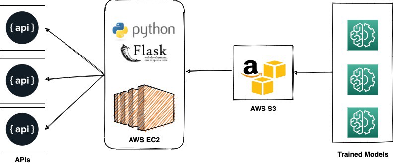
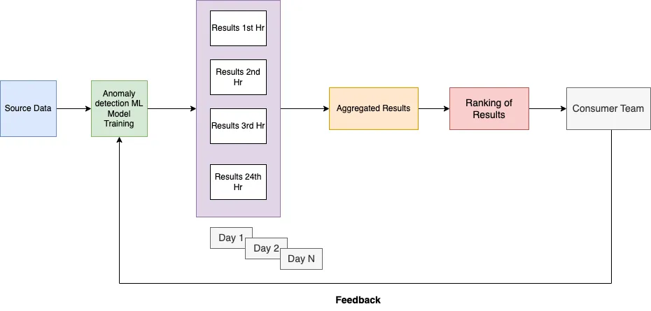
The current process looks like this.</p>

<p><img src="http://aditya00kumar.github.io//assets/image/ML_model_deployment.jpeg" alt="ML model deployment" /></p>

<h2 id="properties-of-the-ranking-function">Properties of the Ranking function</h2>

<p>We want to achieve the following properties from the ranking function. These properties are more tailored to my use case but can be easily modified based on the problem and needs</p>

<ol>
  <li>A score between 0 to 1. A score closer to 1 means a higher priority and vice versa.</li>
  <li>More weightage to the anomalies that occurs multiple times within a time frame.</li>
  <li>Scale the score of the anomaly if it was detected before by the ML model. Recently detected anomalies need to be weighted more compared to the anomaly that was detected before.</li>
  <li>Consider the consumer team’s feedback on already checked responses and incorporate that into your ML system.</li>
</ol>

<h2 id="ranking-function">Ranking Function</h2>

<p>We will consider the ranking function in two parts:</p>

<ol>
  <li><strong>Baseline Ranking function</strong>: The baseline ranking function provides a score for the detected anomalies. There can be multiple approaches to it but will consider frequency-based approaches in this blog post to keep it simple and complete.</li>
  <li><strong>Weighing Function for historical detections</strong>: The weighing function is a parameter that will include the historical score at a discounted factor.</li>
</ol>

<h2 id="baseline-ranking-function">Baseline Ranking function</h2>

<ol>
  <li>
    <p><strong>Step function</strong>: The idea behind this approach is to use the frequency of occurrence of an anomaly as the ranking measure, i.e. if one anomaly appears multiple times in the result, then should be ranked higher than any anomaly which appears less number of times in the result. The score of the function needs to be in the range of <code class="language-plaintext highlighter-rouge">[0,1]</code> , we can divide the final score of anomaly by <code class="language-plaintext highlighter-rouge">max_value</code> so that score will lie in the desired range. <code class="language-plaintext highlighter-rouge">Ranking_anomaly = F(frequency_anomaly, max_value)</code></p>
  </li>
  <li>
    <p><strong>Sigmoid Function</strong></p>
  </li>
</ol>

<p><img src="http://aditya00kumar.github.io//assets/image/Sigmoid_Function.jpeg" alt="Sigmoid Function" /></p>

<p><img src="http://aditya00kumar.github.io//assets/image/Sigmoid_Graph.jpeg" alt="Sigmoid Graph" />
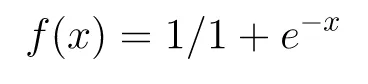
The sigmoid function is widely used in ML and the range of this function is already in
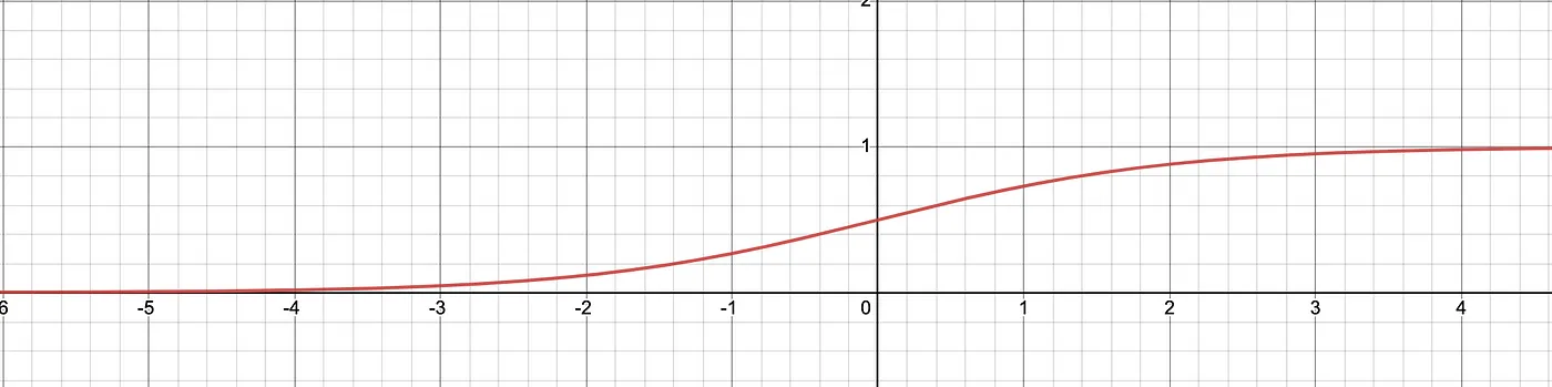
 <code class="language-plaintext highlighter-rouge">[0,1]</code>. This function has some properties that need to be modified to adapt it to our needs i.e
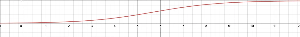
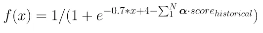
</p>

<ul>
  <li><code class="language-plaintext highlighter-rouge">𝜎(x) → 0 as, x → ≤-4</code> , we want the score to be as close to 0 when x → 0, therefore the range of this function needs to be shifted to the right by 4 units.</li>
  <li><code class="language-plaintext highlighter-rouge">𝜎(x) → 1 as, x → ≥ 3</code> i.e. the value of x greater than 3 will be close to 1, we need to scale this function to reach a score close to 1 when let’s say we have at least 10 anomalies. i.e. function needs to be scaled by 0.7</li>
</ul>

<p>Also in our case, if an anomaly is detected 10 times is as important as if it is detected 24 times in a day and still the score for the latter is greater than the former (although the magnitude is significantly less) and that is precisely what we want.</p>

<p>Now the equation becomes</p>

<p><img src="http://aditya00kumar.github.io//assets/image/Modified_Sigmoid_function.jpeg" alt="Modified Sigmoid function" /></p>

<p>
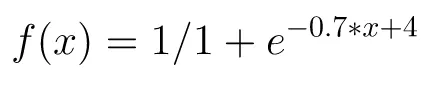
and the graph looks like this</p>

<p><img src="http://aditya00kumar.github.io//assets/image/Modified_Sigmoid_function_graph.jpeg" alt="Modified Sigmoid function graph" /></p>

<p>Both of the above approaches work fine for most cases, but this one doesn’t account for the historical detections by the ML model for more than 1 day. To consider anomalies which are detected previously i.e. not on the same day, we can define some constant values for the historical detections. We want to give more weightage to anomalies that have been detected recently.</p>

<h3 id="weighing-function-for-historical-detections">Weighing Function for historical detections</h3>

<p>The idea here is to use a function that accounts for the score for the historical detections. We will use 𝛼 to denote this, basically in this case the whole equation will become something like this</p>

<p><img src="http://aditya00kumar.github.io//assets/image/Ranking_with_the_historical_score.jpeg" alt="Ranking with the historical score" /></p>

<ul>
  <li><strong>
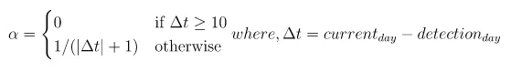
Constant value for discounted historical score</strong>: Any value in the range <code class="language-plaintext highlighter-rouge">[0,1)</code> will discount the score. This score can be adjusted based on the requirements and use case. There can be a different variation of this score, one variation is having separate weights for each day i.e. 0.8 for a 1-day difference, 0.3 for a 2-day difference, etc. Another variation can be defined by equal weight to each day and can be changed based on the needs and underlying problem to be solved. This can be easily implemented by maintaining a data structure that keeps the weights for each day and multiplying the score with this weight.</li>
  <li><strong>Time decay factor</strong>: This function will give more weight to recently detected anomalies and less weight to the anomalies detected earlier.</li>
</ul>

<p><img src="http://aditya00kumar.github.io//assets/image/historical_weights_for_detected_anomalies.jpeg" alt="historical weights for detected anomalies" /></p>

<p><img src="http://aditya00kumar.github.io//assets/image/Graph_1.jpeg" alt="Graph" /></p>

<h3 id="how-long-will-it-take-to-diminish-the-effect-of-an-entry-in-the-result">
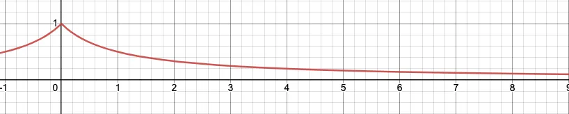
How long will it take to diminish the effect of an entry in the result?</h3>

<p>This value of 𝛼 discounts scores at a rate of 0.5 i.e. for every day passed it changes the score to half. Small scores will vanish very quickly and larger scores will take a few days to come close to 0.</p>

<h2 id="implementation">Implementation</h2>

<p>This can be easily implemented in any database using SQL queries and can be scheduled as tasks. Anomaly detected are stored in a table with the timestamp which helps in tracking how many anomalies are generated in a particular hour or day. So finally the problem comes down to “how to write the above-explained ranking function?”.</p>

<p>
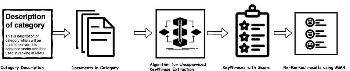
The idea is to bring the previously ranked anomalies to one intermediate table and sum up the score of the current day with the historical score by joining the whole table. The historical score can be adjusted based on the flavor of the ranking function you want to use. Visually it can be understood as below figure</p>

<p><img src="http://aditya00kumar.github.io//assets/image/Implementation_Ranking_function.jpeg" alt="Implementation of the Ranking function" /></p>

<p>
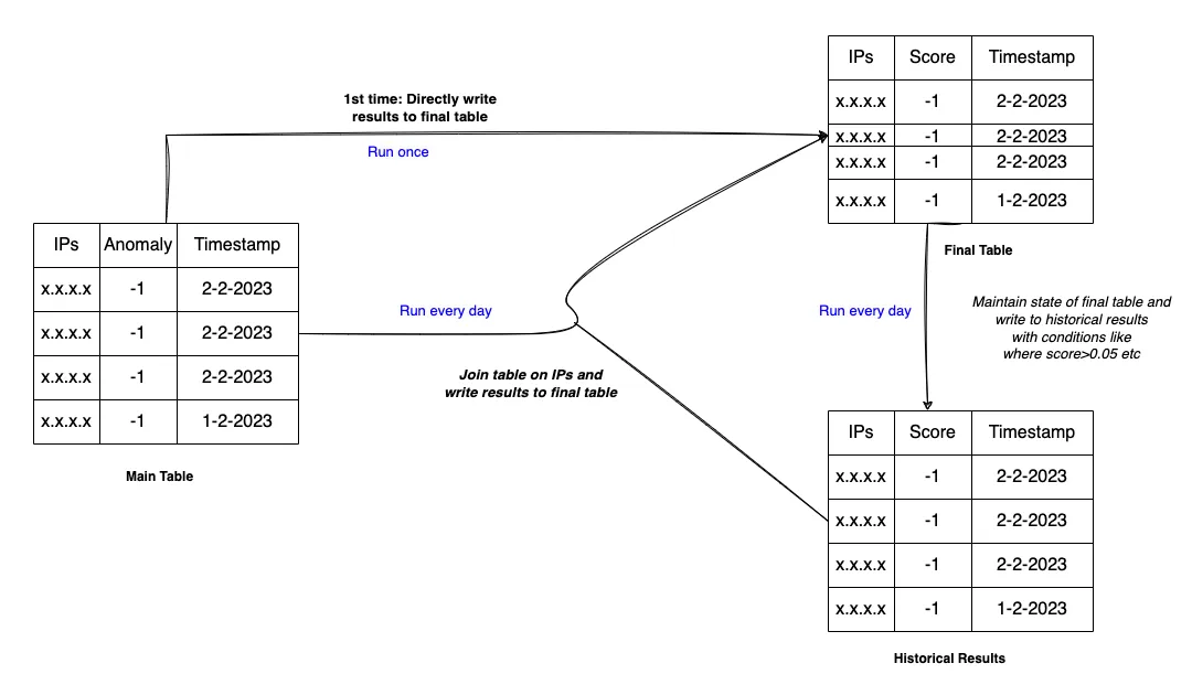
Each run can be scheduled as a task at a regular cadence based on the requirement. The consumer team can start looking at the anomalies and do the investigation based on the updated score from the historical data. Feedback from the team can be directly incorporated into the system either via a ranking function or can be used to filter data while training the ML model or at inference time. These decisions can be taken accordingly based on need and use case.</p>

<p>Please let me know if you like the post, or have some suggestions/concerns and feel free to reach out to me on <a href="https://www.linkedin.com/in/aditya00kumar/">LinkedIn</a>.</p>

<p><strong>References</strong>:</p>

<ol>
  <li><a href="https://docs.snowflake.com/en/user-guide/tasks-intro">https://docs.snowflake.com/en/user-guide/tasks-intro</a></li>
</ol>]]></content><author><name>Aditya Kumar</name></author><category term="Machine Learning, Model Monitoring, Ranking Results" /><category term="post" /><category term="Machine learning" /><category term="Ranking" /><category term="Anomaly detection" /><summary type="html"><![CDATA[In this blog post, I will go through one of the problems I have recently faced that seems to be reoccurring in some form or another, which requires a ranking of the results produced by machine learning models in absence of implicit, explicit, or delayed feedback. I will explain the background, and problem and then discuss the approaches that can be used to solve the problem. And finally, how it can be easily implemented in any database and can be scheduled as a task in DB.]]></summary></entry><entry><title type="html">Monitoring Machine Learning Models in Production</title><link href="http://aditya00kumar.github.io//2021/03/02/Blog.html" rel="alternate" type="text/html" title="Monitoring Machine Learning Models in Production" /><published>2021-03-02T00:00:00+00:00</published><updated>2021-03-09T19:25:52+00:00</updated><id>http://aditya00kumar.github.io//2021/03/02/Blog</id><content type="html" xml:base="http://aditya00kumar.github.io//2021/03/02/Blog.html"><![CDATA[<p>After deploying many ML models in production, it became evident that there should be an easy and efficient way to monitor the ML models after deployment. This blog post is focused on monitoring the classification models in production.</p>

<p>Recently, I was working on the text classification problem which will classify the text into one of ~50 categories. Once the model is built and tested, it needs to be deployed as a flask API along with other models. Some text classification models are already deployed as an API that uses python flask to serve the incoming requests which use Gunicorn as a WSGI server and are deployed on Kubernetes clusters and trained models are stored in S3.<!--more--> So, the current architecture looks something like this, and a newly trained model needs to be deployed in this kind of setup</p>

<p><img src="http://aditya00kumar.github.io//assets/image/Archicture.jpeg" alt="Classification Model APIs" /></p>

<p>To prepare the training data, we have started with some keywords related to categories to tag the data, generate new keywords from existing categories, manually tagging data, etc to prepare the training dataset. Handling cases, where a text might fall into any of closely related categories and also considered already deployed classifiers to tag data in some of the categories on which they were trained on. Random manual check on labels was done to ensure if tagged entries using the above methods are good enough as training data is in the range of few millions.</p>

<p>Then a model is trained using training data and tested on a held-out set to measure the performance of the classifier, if model performance is acceptable on test data then the model is deployed in production as an API. Now as the model is deployed, then why there is a need for monitoring the model?</p>

<p><strong>Need for monitoring</strong></p>

<p>You have already put the classification model in production, which performed very well on your test dataset. But,</p>

<ul>
  <li>How do you know that the model is performing well on the new data?</li>
  <li>How do you know it is time to retrain the model?</li>
  <li>How to know the effect of data drift and conceptual drift on the model?</li>
</ul>

<p>One possible way to detect the performance of the classifier is to take all incoming requests for classification for a certain duration and manually label the data and compare it with model predictions. Do this exercise periodically after a certain period of time to gauge the performance of the model. This is the same thing that we did while training the model and needs to be done periodically. This process seems unintuitive to me and requires a lot of manual effort and periodically monitoring of models which become very cumbersome when you have many classification models running in production.</p>

<p>There is a need for something simple, quick, and yet very intuitive which gives an idea about how models are performing in the production. Also in the current setup, how models are deployed and used by downstream applications is pretty stable, therefore don’t want to invest too much time in getting a look at available ML tools that provides this functionality out of the box.</p>

<p><strong>Prediction Distribution of Model</strong></p>

<p>After some research, having a dashboard that displays the plot for the prediction distribution of the incoming requests seems very intuitive to me and will also answer some of the questions, like:</p>

<ul>
  <li>How a model is performing against each category?</li>
  <li>Does prediction distribution follow a similar pattern as training data?</li>
  <li>Is the model biased towards any category i.e. model is predicting some class very often?</li>
  <li>Is the model failing to predict any category?</li>
  <li>Is there a need to retrain the model?</li>
</ul>

<p><img src="http://aditya00kumar.github.io//assets/image/BERT_class_Prediction.png" alt="Distribution of predicted classes" /></p>

<p><strong>What else can be tracked?</strong></p>

<p>A new model is trained to predict the text into one of the 52 categories and uses the BERT-base-cased model, so to deploy that in production and staging we have to increase the resources significantly in comparison to previous models so that model can run smoothly on CPU.</p>

<p>Generally, when it comes to deployment, there are two environments Staging/UAT and Prod, and there is a significant difference in these environments in terms of resources allocated to the application like memory, CPU time. The idea is to allocate more resources to the application in production so that it can serve its purpose without any issue. In our case also, in production number of workers running are 2X times as of staging environment, hence resources needed are also doubled. Therefore we want to know that do we really need the increased resources in production?</p>

<p>That’s why we want to track the number of API calls which will eventually answer a few questions like</p>

<ul>
  <li>Is there any need to increase or decrease the resources in production?</li>
  <li>Can the whole system be deployed as batch inference in case the number of API calls is less?</li>
  <li>Are previously deployed models still being used by downstream applications and if so, then how frequent?</li>
</ul>

<p><img src="http://aditya00kumar.github.io//assets/image/API_Calls.png" alt="Total API Calls" /></p>

<p>There might be some more metrics we can measure like, the responsiveness of APIs. But here, the main focus was to know how the model was performing in predicting the categories and keep the effort very simple to track down these metrics.</p>

<p>Here is the sample code for generating divs for Bar plot.</p>

<div class="language-python highlighter-rouge"><div class="highlight"><pre class="highlight"><code><span class="kn">import</span> <span class="nn">plotly</span>
<span class="kn">import</span> <span class="nn">plotly.express</span> <span class="k">as</span> <span class="n">px</span>

<span class="k">def</span> <span class="nf">generate_div</span><span class="p">(</span><span class="n">prediction_distribution</span><span class="p">):</span>
    <span class="s">"""
    function to generate div html tags from model prediction distribution dictionary.
    :param prediction_distribution: dictionary with keys as model name and its values as a dictionary having 
    its classes and values. It should look like:
    {'1.0': {'Class 1': 23,
         'Class 2': 19,
         'Class 3: 40},
    '2.0': {'Category 1': 10,
         'Category 2': 42,
         'Category 3': 23,
         'Category 4': 20,
         },
    '3.0': {'Class A': 10,
         'Class B': 23,
         'Class C': 12,
         }}
    :type prediction_distribution: Dictionary
    :return: html div tags
    :rtype: list of div tags
    """</span>
    <span class="n">divs</span> <span class="o">=</span> <span class="p">[]</span>
    <span class="k">for</span> <span class="n">version</span> <span class="ow">in</span> <span class="n">prediction_distribution</span><span class="p">:</span>
        <span class="n">the_dict</span> <span class="o">=</span> <span class="p">{</span><span class="s">'Intent_categories'</span><span class="p">:[],</span> <span class="s">'Values'</span><span class="p">:[]}</span>
        <span class="n">the_dict</span><span class="p">[</span><span class="s">'Intent_categories'</span><span class="p">]</span> <span class="o">=</span> <span class="nb">list</span><span class="p">(</span><span class="n">prediction_distribution</span><span class="p">[</span><span class="n">version</span><span class="p">].</span><span class="n">keys</span><span class="p">())</span>
        <span class="n">the_dict</span><span class="p">[</span><span class="s">'Values'</span><span class="p">]</span> <span class="o">=</span> <span class="p">[</span><span class="n">prediction_distribution</span><span class="p">[</span><span class="n">version</span><span class="p">][</span><span class="n">i</span><span class="p">]</span> <span class="k">for</span> <span class="n">i</span> <span class="ow">in</span> <span class="n">the_dict</span><span class="p">[</span><span class="s">'Intent_categories'</span><span class="p">]]</span>
        <span class="n">fig</span> <span class="o">=</span> <span class="n">px</span><span class="p">.</span><span class="n">bar</span><span class="p">(</span><span class="n">the_dict</span><span class="p">,</span> <span class="n">x</span><span class="o">=</span><span class="s">'Intent_categories'</span><span class="p">,</span> <span class="n">y</span><span class="o">=</span><span class="s">'Values'</span><span class="p">,</span> <span class="n">color</span><span class="o">=</span><span class="s">'Values'</span><span class="p">,</span><span class="n">title</span><span class="o">=</span><span class="s">"Class prediction distribution for model %s"</span><span class="o">%</span><span class="n">version</span><span class="p">)</span>
        <span class="n">fig</span><span class="p">.</span><span class="n">update_layout</span><span class="p">(</span><span class="n">uniformtext_minsize</span><span class="o">=</span><span class="mi">8</span><span class="p">,</span> <span class="n">uniformtext_mode</span><span class="o">=</span><span class="s">'hide'</span><span class="p">,</span> <span class="n">xaxis_tickangle</span><span class="o">=</span><span class="mi">45</span><span class="p">)</span>
        <span class="n">divs</span><span class="p">.</span><span class="n">append</span><span class="p">(</span><span class="n">plotly</span><span class="p">.</span><span class="n">io</span><span class="p">.</span><span class="n">to_html</span><span class="p">(</span><span class="n">fig</span><span class="p">,</span> <span class="n">include_plotlyjs</span><span class="o">=</span><span class="bp">False</span><span class="p">,</span> <span class="n">full_html</span><span class="o">=</span><span class="bp">False</span><span class="p">))</span>
    <span class="k">return</span> <span class="n">divs</span>
</code></pre></div></div>

<p>Below, HTML template can be rendered from the Flask module by passing the HTML divs generated by the above code.</p>

<div class="language-python highlighter-rouge"><div class="highlight"><pre class="highlight"><code><span class="o">@</span><span class="n">app</span><span class="p">.</span><span class="n">route</span><span class="p">(</span><span class="s">"/monitoring"</span><span class="p">,</span> <span class="n">methods</span><span class="o">=</span><span class="p">[</span><span class="s">'GET'</span><span class="p">])</span>
<span class="k">def</span> <span class="nf">monitor</span><span class="p">():</span>
    <span class="n">divs</span> <span class="o">=</span> <span class="n">generate_div</span><span class="p">(</span><span class="n">predict_dist</span><span class="p">)</span>
    <span class="k">return</span> <span class="n">render_template</span><span class="p">(</span><span class="s">'monitor.html'</span><span class="p">,</span> <span class="n">div1</span><span class="o">=</span><span class="n">Markup</span><span class="p">(</span><span class="n">divs</span><span class="p">[</span><span class="mi">0</span><span class="p">]),</span>   <span class="n">div2</span><span class="o">=</span><span class="n">Markup</span><span class="p">(</span><span class="n">divs</span><span class="p">[</span><span class="mi">1</span><span class="p">]),</span> <span class="n">div3</span><span class="o">=</span><span class="n">Markup</span><span class="p">(</span><span class="n">divs</span><span class="p">[</span><span class="mi">2</span><span class="p">]))</span>

</code></pre></div></div>

<div class="language-html highlighter-rouge"><div class="highlight"><pre class="highlight"><code><span class="nt">&lt;html&gt;</span>
   <span class="nt">&lt;head&gt;</span>
      <span class="c">&lt;!-- Plotly.js --&gt;</span>
      <span class="nt">&lt;script </span><span class="na">src=</span><span class="s">"https://cdn.plot.ly/plotly-latest.min.js"</span><span class="nt">&gt;&lt;/script&gt;</span>
      <span class="nt">&lt;style&gt;</span> 
         <span class="nf">#myDIV</span> <span class="p">{</span>
         <span class="nl">border</span><span class="p">:</span> <span class="m">1px</span> <span class="nb">solid</span> <span class="no">black</span><span class="p">;</span>
         <span class="nl">background-color</span><span class="p">:</span> <span class="no">lightblue</span><span class="p">;</span>
         <span class="nl">width</span><span class="p">:</span> <span class="nb">auto</span><span class="p">;</span>
         <span class="nl">overflow</span><span class="p">:</span> <span class="nb">auto</span><span class="p">;</span>
         <span class="p">}</span>
      <span class="nt">&lt;/style&gt;</span>
   <span class="nt">&lt;/head&gt;</span>
   <span class="nt">&lt;body&gt;</span>
      <span class="nt">&lt;h1&gt;</span>Model Monitoring<span class="nt">&lt;/h1&gt;</span>
      <span class="nt">&lt;table</span> <span class="na">style=</span><span class="s">"width:100%"</span><span class="nt">&gt;</span>
         <span class="nt">&lt;tr&gt;</span>
            <span class="nt">&lt;td&gt;&lt;/td&gt;</span>
         <span class="nt">&lt;/tr&gt;</span>
         <span class="nt">&lt;tr&gt;</span>
            <span class="nt">&lt;td&gt;&lt;/td&gt;</span>
            <span class="nt">&lt;td&gt;&lt;/td&gt;</span>
         <span class="nt">&lt;/tr&gt;</span>
      <span class="nt">&lt;/table&gt;</span>
   <span class="nt">&lt;/body&gt;</span>
<span class="nt">&lt;/html&gt;</span>
</code></pre></div></div>

<p>Please let me know if you like the post, or have some suggestions/concerns and feel free to reach out to me on <a href="https://www.linkedin.com/in/aditya00kumar/">LinkedIn</a>.</p>

<p><strong>References</strong>:</p>
<ol>
  <li>https://christophergs.com/machine%20learning/2020/03/14/how-to-monitor-machine-learning-models/</li>
  <li>https://mlinproduction.com/value-propositions-ml-monitoring-system/</li>
  <li>https://www.explorium.ai/blog/understanding-and-handling-data-and-concept-drift/</li>
</ol>]]></content><author><name>Aditya Kumar</name></author><category term="Machine Learning, Model Monitoring" /><category term="post" /><category term="Machine learning" /><category term="NLP" /><category term="Model Monitoring" /><category term="Code" /><summary type="html"><![CDATA[After deploying many ML models in production, it became evident that there should be an easy and efficient way to monitor the ML models after deployment. This blog post is focused on monitoring the classification models in production. Recently, I was working on the text classification problem which will classify the text into one of ~50 categories. Once the model is built and tested, it needs to be deployed as a flask API along with other models. Some text classification models are already deployed as an API that uses python flask to serve the incoming requests which use Gunicorn as a WSGI server and are deployed on Kubernetes clusters and trained models are stored in S3.]]></summary></entry><entry><title type="html">Wilson Lower bound Score and Bayesian Approximation for K star scale rating to Rate products</title><link href="http://aditya00kumar.github.io//2020/01/16/Blog.html" rel="alternate" type="text/html" title="Wilson Lower bound Score and Bayesian Approximation for K star scale rating to Rate products" /><published>2020-01-16T00:00:00+00:00</published><updated>2017-03-09T19:25:52+00:00</updated><id>http://aditya00kumar.github.io//2020/01/16/Blog</id><content type="html" xml:base="http://aditya00kumar.github.io//2020/01/16/Blog.html"><![CDATA[<script type="text/javascript" async="" src="https://cdn.mathjax.org/mathjax/latest/MathJax.js?config=TeX-MML-AM_CHTML">
</script>

<p>As a maintainer of an online community, which is having a lot of  products where user gives a rating to products based on their  experience, then it is definite that at some point you have to find an  answer to questions like</p>
<ul>
  <li>How you are going to show the product on the  page based on filters i.e. like highest voted or lowest voted, etc.?<!--more--> Or</li>
  <li>How can you rate a product based on upvotes and downvotes?</li>
  <li>How you can  give a score to a product which is rated on a K scale by users?</li>
</ul>

<p>There are some ways you can find a score and rate products accordingly:</p>

<ol>
  <li><code class="language-plaintext highlighter-rouge">Score = Average rating of products</code></li>
  <li><code class="language-plaintext highlighter-rouge">Score = Positive rating - Negative rating</code></li>
  <li><code class="language-plaintext highlighter-rouge">Score = Proportion of Positive ratings</code></li>
</ol>

<p>Evan Miller’s famous blog <a href="http://www.evanmiller.org/how-not-to-sort-by-average-rating.html">How not to sort</a>, explains why  the above two scores are not good ways to rate the product or sort a product.</p>

<p>Lower bound of <strong><code class="language-plaintext highlighter-rouge">Wilson score confidence interval for a Bernoulli parameter</code></strong> provides a way to sort a product based on positive and negative ratings.</p>

<p>The idea here is to treat the existing set of user ratings as a statistical sampling of a hypothetical set of user ratings from all users and then use this score. In other words, what user community would think about upvoting a product with 95% confidence given that we have an existing rating for this product with a sample (subset from the whole community) user ratings.</p>

<p>Therefore if we know what a sample population thinks i.e. user reviews for a product, you can use this to estimate the preferences of the whole community.</p>

<p>If there are <code class="language-plaintext highlighter-rouge">X</code> positive votes  and <code class="language-plaintext highlighter-rouge">Y</code> negative votes for a product and we want to understand how popular the product will be across the whole community. We can estimate that with 95% confidence between <code class="language-plaintext highlighter-rouge">wilson_lower_bound_score</code> and <code class="language-plaintext highlighter-rouge">wilson_upper_bound_score</code>% of users will upvote this product using Wilson Score of confidence interval.</p>

<h3 id="wilson-score">Wilson Score</h3>

<p><img src="https://latex.codecogs.com/png.latex?\fn_jvn&space;\left(\hat{p}&plus;\frac{z_{\alpha&space;/&space;2}^{2}}{2&space;n}&space;\pm&space;z_{\alpha&space;/&space;2}&space;\sqrt{\left[\hat{p}(1-\hat{p})&plus;z_{\alpha&space;/&space;2}^{2}&space;/&space;4&space;n\right]&space;/&space;n}\right)&space;/\left(1&plus;z_{\alpha&space;/&space;2}^{2}&space;/&space;n\right)" /></p>

<p>where,
    \(\hat{p}\)=<code class="language-plaintext highlighter-rouge">(# of positive ratings)/(Total ratings)</code> <br />
    \(n\) <code class="language-plaintext highlighter-rouge">= Total ratings</code><br />
    \(z_{α/2}\)= <code class="language-plaintext highlighter-rouge">quantile of the standard normal distribution</code></p>

<div class="language-python highlighter-rouge"><div class="highlight"><pre class="highlight"><code><span class="kn">import</span> <span class="nn">math</span>
<span class="kn">import</span> <span class="nn">scipy.stats</span> <span class="k">as</span> <span class="n">st</span>

<span class="k">def</span> <span class="nf">wilson_lower_bound</span><span class="p">(</span><span class="n">pos</span><span class="p">,</span> <span class="n">n</span><span class="p">,</span> <span class="n">confidence</span><span class="o">=</span><span class="mf">0.95</span><span class="p">):</span>
    <span class="s">"""
    Function to provide lower bound of wilson score
    :param pos: No of positive ratings
    :param n: Total number of ratings
    :param confidence: Confidence interval, by default is 95 %
    :return: Wilson Lower bound score
    """</span>
    <span class="k">if</span> <span class="n">n</span> <span class="o">==</span> <span class="mi">0</span><span class="p">:</span>
        <span class="k">return</span> <span class="mi">0</span>
    <span class="n">z</span> <span class="o">=</span> <span class="n">st</span><span class="p">.</span><span class="n">norm</span><span class="p">.</span><span class="n">ppf</span><span class="p">(</span><span class="mi">1</span> <span class="o">-</span> <span class="p">(</span><span class="mi">1</span> <span class="o">-</span> <span class="n">confidence</span><span class="p">)</span> <span class="o">/</span> <span class="mi">2</span><span class="p">)</span>
    <span class="n">phat</span> <span class="o">=</span> <span class="mf">1.0</span> <span class="o">*</span> <span class="n">pos</span> <span class="o">/</span> <span class="n">n</span>
    <span class="k">return</span> <span class="p">(</span><span class="n">phat</span> <span class="o">+</span> <span class="n">z</span> <span class="o">*</span> <span class="n">z</span> <span class="o">/</span> <span class="p">(</span><span class="mi">2</span> <span class="o">*</span> <span class="n">n</span><span class="p">)</span> <span class="o">-</span> <span class="n">z</span> <span class="o">*</span> <span class="n">math</span><span class="p">.</span><span class="n">sqrt</span><span class="p">((</span><span class="n">phat</span> <span class="o">*</span> <span class="p">(</span><span class="mi">1</span> <span class="o">-</span> <span class="n">phat</span><span class="p">)</span> <span class="o">+</span> <span class="n">z</span> <span class="o">*</span> <span class="n">z</span> <span class="o">/</span> <span class="p">(</span><span class="mi">4</span> <span class="o">*</span> <span class="n">n</span><span class="p">))</span> <span class="o">/</span> <span class="n">n</span><span class="p">))</span> <span class="o">/</span> <span class="p">(</span><span class="mi">1</span> <span class="o">+</span> <span class="n">z</span> <span class="o">*</span> <span class="n">z</span> <span class="o">/</span> <span class="n">n</span><span class="p">)</span>
</code></pre></div></div>
<p>Wilson Confidence Interval considers binomial distribution for score calculation i.e. it considers only positive and negative ratings. If your product is rated on 5 scale rating, then we can convert ratings {1-3} into negative and {4,5} to positive rating and can calculate wilson score.</p>

<p>Lets look at some examples:</p>

<ol>
  <li>
    <p>If a product is rated across each category uniformly [10, 10, 10, 10, 10], i.e. 10 votes for rating {1-5},  then <code class="language-plaintext highlighter-rouge">wilson_lower_bound(20,50,.95), avg_rating([10, 10, 10, 10, 10]) =&gt; (0.2760838973025655, 3.0)</code></p>
  </li>
  <li>
    <p>A product receives only one rating i.e. positive and one product receives 10 positive and 2 negative ratings: in that case value of product having more ratings should be greater <code class="language-plaintext highlighter-rouge">wilson_lower_bound(1,1,0.95) &lt; wilson_lower_bound(10,12,0.95)</code> , which is true.</p>
  </li>
  <li>
    <p>Product having ratings A: (209 up and 50 down votes) and B: (118 up and 25 down) <code class="language-plaintext highlighter-rouge">wilson_lower_bound(209,259,0.95) &lt; wilson_lower_bound(118,143,0.95)</code></p>
  </li>
  <li>
    <p>Suppose one product receives [5, 10, 20, 0, 0] ratings, then <code class="language-plaintext highlighter-rouge">wilson_lower_bound(0,35,0.95) = 0</code>, If any product  does not have any positive ratings associated with it then the Wilson score is zero.</p>
  </li>
  <li>
    <p>Wilson Score can not be applied to new product which is yet to receive any rating, if using above implementation <code class="language-plaintext highlighter-rouge">wilson_lower_bound(0,0,0.95) = 0</code>.</p>

    <p>Wilson score gives us the zero value for both the product which does not received any positive user rating and to product which is new and yet to receive any rating, which essentially does not make any sense as this implies <strong>no user rated product</strong> is same as <strong>product having lower ratings</strong>. Also, it is not clear how tight the lower bound is i.e., how far it deviates away from the “real” proportion of thumb-ups [1]. It does not seem intuitive to convert items rated on five star scale to convert to up votes and down votes for calculating scores to follow binomial distribution.</p>
  </li>
</ol>

<h2 id="bayesian-approximation">Bayesian Approximation</h2>

<p><strong>Bayesian Approximation</strong> provides a way to give a score to product when they are rated on star scale.</p>

<p><img src="https://latex.codecogs.com/png.latex?\fn_jvn&space;\large&space;\left(\hat{p}&plus;\frac{z_{\alpha&space;/&space;2}^{2}}{2&space;n}&space;\pm&space;z_{\alpha&space;/&space;2}&space;\sqrt{\left[\hat{p}(1-\hat{p})&plus;z_{\alpha&space;/&space;2}^{2}&space;/&space;4&space;n\right]&space;/&space;n}\right)&space;/\left(1&plus;z_{\alpha&space;/&space;2}^{2}&space;/&space;n\right)" title="\large \left(\hat{p}&plus;\frac{z_{\alpha&space;/&space;2}^{2}}{2&space;n}&space;\pm&space;z_{\alpha&space;/&space;2}&space;\sqrt{\left[\hat{p}(1-\hat{p})&plus;z_{\alpha&space;/&space;2}^{2}&space;/&space;4&space;n\right]&space;/&space;n}\right)&space;/\left(1&plus;z_{\alpha&space;/&space;2}^{2}&space;/&space;n\right)" /></p>

<p>where, \(s_k=k\) (That is, 1 point, 2 points, ….) <br />
      \(N\) = total ratings, with \(n_k\) ratings for \(k^{th}\) scale</p>

<p>The above expression provides the lower bound of a normal approximation to a Bayesian credible interval for the average rating. For more mathematical details please check [4].</p>
<div class="language-python highlighter-rouge"><div class="highlight"><pre class="highlight"><code><span class="kn">import</span> <span class="nn">math</span>
<span class="kn">import</span> <span class="nn">scipy.stats</span> <span class="k">as</span> <span class="n">st</span>

<span class="k">def</span> <span class="nf">bayesian_rating_products</span><span class="p">(</span><span class="n">n</span><span class="p">,</span> <span class="n">confidence</span><span class="o">=</span><span class="mf">0.95</span><span class="p">):</span>
    <span class="s">"""
    Function to calculate wilson score for N star rating system. 
    :param n: Array having count of star ratings where ith index represent the votes for that category i.e. [3, 5, 6, 7, 10]
    here, there are 3 votes for 1-star rating, similarly 5 votes for 2-star rating. 
    :param confidence: Confidence interval
    :return: Score
    """</span>
    <span class="k">if</span> <span class="nb">sum</span><span class="p">(</span><span class="n">n</span><span class="p">)</span><span class="o">==</span><span class="mi">0</span><span class="p">:</span>
        <span class="k">return</span> <span class="mi">0</span>
    <span class="n">K</span> <span class="o">=</span> <span class="nb">len</span><span class="p">(</span><span class="n">n</span><span class="p">)</span>
    <span class="n">z</span> <span class="o">=</span> <span class="n">st</span><span class="p">.</span><span class="n">norm</span><span class="p">.</span><span class="n">ppf</span><span class="p">(</span><span class="mi">1</span> <span class="o">-</span> <span class="p">(</span><span class="mi">1</span> <span class="o">-</span> <span class="n">confidence</span><span class="p">)</span> <span class="o">/</span> <span class="mi">2</span><span class="p">)</span>
    <span class="n">N</span> <span class="o">=</span> <span class="nb">sum</span><span class="p">(</span><span class="n">n</span><span class="p">)</span>
    <span class="n">first_part</span> <span class="o">=</span> <span class="mf">0.0</span>
    <span class="n">second_part</span> <span class="o">=</span> <span class="mf">0.0</span>
    <span class="k">for</span> <span class="n">k</span><span class="p">,</span> <span class="n">n_k</span> <span class="ow">in</span> <span class="nb">enumerate</span><span class="p">(</span><span class="n">n</span><span class="p">):</span>
        <span class="n">first_part</span> <span class="o">+=</span> <span class="p">(</span><span class="n">k</span><span class="o">+</span><span class="mi">1</span><span class="p">)</span><span class="o">*</span><span class="p">(</span><span class="n">n</span><span class="p">[</span><span class="n">k</span><span class="p">]</span><span class="o">+</span><span class="mi">1</span><span class="p">)</span><span class="o">/</span><span class="p">(</span><span class="n">N</span><span class="o">+</span><span class="n">K</span><span class="p">)</span>
        <span class="n">second_part</span> <span class="o">+=</span> <span class="p">(</span><span class="n">k</span><span class="o">+</span><span class="mi">1</span><span class="p">)</span><span class="o">*</span><span class="p">(</span><span class="n">k</span><span class="o">+</span><span class="mi">1</span><span class="p">)</span><span class="o">*</span><span class="p">(</span><span class="n">n</span><span class="p">[</span><span class="n">k</span><span class="p">]</span><span class="o">+</span><span class="mi">1</span><span class="p">)</span><span class="o">/</span><span class="p">(</span><span class="n">N</span><span class="o">+</span><span class="n">K</span><span class="p">)</span>
    <span class="n">score</span> <span class="o">=</span> <span class="n">first_part</span> <span class="o">-</span> <span class="n">z</span> <span class="o">*</span> <span class="n">math</span><span class="p">.</span><span class="n">sqrt</span><span class="p">((</span><span class="n">second_part</span> <span class="o">-</span> <span class="n">first_part</span><span class="o">*</span><span class="n">first_part</span><span class="p">)</span><span class="o">/</span><span class="p">(</span><span class="n">N</span><span class="o">+</span><span class="n">K</span><span class="o">+</span><span class="mi">1</span><span class="p">))</span>
    <span class="k">return</span> <span class="n">score</span>
</code></pre></div></div>

<p>Lets look at some test samples</p>

<ol>
  <li>
    <p><code class="language-plaintext highlighter-rouge">bayesian_rating_products([0, 0, 0, 0, 1]) = 2.2290</code></p>
  </li>
  <li>
    <p><code class="language-plaintext highlighter-rouge">bayesian_rating_products([0, 2, 0, 10, 0]) = 2.9921</code></p>
  </li>
  <li>
    <p><code class="language-plaintext highlighter-rouge">bayesian_rating_products([5, 10, 20, 0, 0]) = 2.2349</code></p>
  </li>
  <li>
    <p><code class="language-plaintext highlighter-rouge">bayesian_rating_products([10, 10, 10, 10, 10]) = 2.6296</code></p>

    <p>On comparing 1 and 2, we can observe the second product should have a higher score and that is the case here. Also in point 3, unlike Wilson score it provides a score to the product which does not have a positive rating and still that score is greater than the first product which seems reasonable to me.</p>

    <p>Bayesian Approximation does not consider only upvotes unlike Wilson’s  score but considers ratings across the K scale and proves to be better  in this scenario.</p>

    <p>Please let me know if you like the post, or have some suggestions/concerns in comments and feel free to reach out to me on <a href="https://www.linkedin.com/in/aditya00kumar/">LinkedIn</a>.</p>
  </li>
</ol>

<h3 id="references">References</h3>

<ol>
  <li><a href="http://www.dcs.bbk.ac.uk/~dell/publications/dellzhang_ictir2011.pdf">How to Count Thumb-Ups and Thumb-Downs: User-Rating based Ranking of Items from an Axiomatic Perspective</a></li>
  <li><a href="https://static.googleusercontent.com/media/research.google.com/en//pubs/archive/36265.pdf">Star Quality: Aggregating Reviews to Rank Products and Merchants</a></li>
  <li>http://www.evanmiller.org/how-not-to-sort-by-average-rating.html</li>
  <li>http://www.evanmiller.org/ranking-items-with-star-ratings.html</li>
</ol>]]></content><author><name>Aditya Kumar</name></author><category term="Ranking, Product Score, Statistics" /><category term="post" /><category term="Machine learning" /><category term="Code" /><summary type="html"><![CDATA[As a maintainer of an online community, which is having a lot of products where user gives a rating to products based on their experience, then it is definite that at some point you have to find an answer to questions like How you are going to show the product on the page based on filters i.e. like highest voted or lowest voted, etc.?]]></summary></entry><entry><title type="html">Maximal Marginal Relevance to Re-rank results in KeyPhrase Extraction</title><link href="http://aditya00kumar.github.io//2019/10/13/Blog.html" rel="alternate" type="text/html" title="Maximal Marginal Relevance to Re-rank results in KeyPhrase Extraction" /><published>2019-10-13T00:00:00+00:00</published><updated>2019-10-13T00:00:00+00:00</updated><id>http://aditya00kumar.github.io//2019/10/13/Blog</id><content type="html" xml:base="http://aditya00kumar.github.io//2019/10/13/Blog.html"><![CDATA[<script type="text/javascript" async="" src="https://cdn.mathjax.org/mathjax/latest/MathJax.js?config=TeX-MML-AM_CHTML">
</script>

<p>Maximal Marginal Relevance a.k.a. MMR has been introduced in this paper <a href="https://www.cs.cmu.edu/~jgc/publication/The_Use_MMR_Diversity_Based_LTMIR_1998.pdf">The Use of MMR, Diversity-Based Reranking for Reordering Documents and Producing Summaries</a>. MMR tries to reduce the redundancy of results while at the same time maintaining query relevance of results for already ranked documents/phrases etc.<!--more--></p>

<p>We first try to understand the scenario by taking an example and will see how MMR is helpful in solving the issue.</p>

<p>Recently I was trying to extract  KeyPhrases from a set of documents that belongs to one category. I have used 
different approaches (TextRank, RAKE, POS tagging, etc.. to name a few) to extract keywords from the documents, which
 provides phrases along with score. This score is used as the ranking of the phrases for that document.</p>

<p>Let’s say your final keyPhrases are ranked like <code class="language-plaintext highlighter-rouge">Good Product, Great Product, Nice Product, Excellent Product, Easy Install, Nice UI, Light weight etc</code>. But there is an issue with this approach, all the phrases like <code class="language-plaintext highlighter-rouge">good product, nice product, excellent product</code> are similar and define the same property of the product and are ranked higher. Suppose we have a space to show just 5 keyPhrases, in that case, we don’t want to show all these similar phrases.</p>

<p>You want to properly utilize this limited space such that the information displayed by the Keyphrases about the documents is diverse enough. Similar types of phrases should not dominate the whole space and users can see a variety of information about the document.</p>

<p><img src="http://aditya00kumar.github.io//assets/image/Keyphrase.png" alt="KeyPhrase Extraction" /></p>

<p>We are going to address this problem in this blog post. There might be different approaches to solve this problem. For the sake of simplicity and completeness of the article, I am going to discuss two approaches:</p>
<ol>
  <li>
    <p><strong>Remove redundant phrases using cosine similarity</strong></p>

    <p>To use <code class="language-plaintext highlighter-rouge">cosine similarity</code> is the naive approach that came to mind to deal with terms having the same meaning. Use word embeddings to find embeddings of phrases and find cosine similarity between embeddings. Set a threshold above which you will consider the terms as similar. Just take one keyPhrase having more score out of clubbed phrases in the result.</p>

    <div class="language-python highlighter-rouge"><div class="highlight"><pre class="highlight"><code> <span class="kn">from</span> <span class="nn">sklearn.metrics.pairwise</span> <span class="kn">import</span> <span class="n">cosine_similarity</span>
 <span class="k">def</span> <span class="nf">club_similar_keywords</span><span class="p">(</span><span class="n">emb_mat</span><span class="p">,</span> <span class="n">sim_score</span><span class="o">=</span><span class="mf">0.9</span><span class="p">):</span>
    <span class="s">"""
    :param emb_mat: matrix having vectors with words as index
    :param sim_score: 0.9 by default
    :return: returns list of unique words from index after combining words which has similarity score of more than
    0.9
    """</span>
    <span class="k">if</span> <span class="nb">len</span><span class="p">(</span><span class="n">emb_mat</span><span class="p">)</span> <span class="o">==</span> <span class="mi">0</span><span class="p">:</span>
        <span class="k">return</span> <span class="s">'NA'</span>
    <span class="n">xx</span> <span class="o">=</span> <span class="n">cosine_similarity</span><span class="p">(</span><span class="n">emb_mat</span><span class="p">)</span>
    <span class="n">final_keywords</span> <span class="o">=</span> <span class="nb">set</span><span class="p">(</span><span class="n">emb_mat</span><span class="p">.</span><span class="n">index</span><span class="p">)</span>
    <span class="n">N</span> <span class="o">=</span> <span class="nb">len</span><span class="p">(</span><span class="n">emb_mat</span><span class="p">.</span><span class="n">index</span><span class="p">)</span>
    <span class="n">dd</span> <span class="o">=</span> <span class="p">{}</span>
    <span class="k">for</span> <span class="n">i</span> <span class="ow">in</span> <span class="nb">range</span><span class="p">(</span><span class="n">N</span><span class="p">):</span>
        <span class="k">for</span> <span class="n">j</span> <span class="ow">in</span> <span class="nb">range</span><span class="p">(</span><span class="n">N</span><span class="p">):</span>
            <span class="k">if</span> <span class="p">(</span><span class="nb">float</span><span class="p">(</span><span class="n">xx</span><span class="p">[</span><span class="n">i</span><span class="p">][</span><span class="n">j</span><span class="p">])</span> <span class="o">&gt;</span> <span class="n">sim_score</span><span class="p">)</span> <span class="ow">and</span> <span class="p">(</span><span class="n">i</span> <span class="o">!=</span> <span class="n">j</span><span class="p">):</span>
                <span class="k">try</span><span class="p">:</span>
                    <span class="n">dd</span><span class="p">[</span><span class="n">emb_mat</span><span class="p">.</span><span class="n">index</span><span class="p">[</span><span class="n">i</span><span class="p">]].</span><span class="n">append</span><span class="p">(</span><span class="n">emb_mat</span><span class="p">.</span><span class="n">index</span><span class="p">[</span><span class="n">j</span><span class="p">])</span>
                <span class="k">except</span><span class="p">:</span>
                    <span class="n">dd</span><span class="p">[</span><span class="n">emb_mat</span><span class="p">.</span><span class="n">index</span><span class="p">[</span><span class="n">i</span><span class="p">]]</span> <span class="o">=</span> <span class="p">[]</span>
                    <span class="n">dd</span><span class="p">[</span><span class="n">emb_mat</span><span class="p">.</span><span class="n">index</span><span class="p">[</span><span class="n">i</span><span class="p">]].</span><span class="n">append</span><span class="p">(</span><span class="n">emb_mat</span><span class="p">.</span><span class="n">index</span><span class="p">[</span><span class="n">j</span><span class="p">])</span>
    <span class="n">removed_keywords</span> <span class="o">=</span> <span class="p">[]</span>
    <span class="k">for</span> <span class="n">key</span> <span class="ow">in</span> <span class="n">dd</span><span class="p">:</span>
        <span class="k">for</span> <span class="n">val</span> <span class="ow">in</span> <span class="n">dd</span><span class="p">[</span><span class="n">key</span><span class="p">]:</span>
            <span class="k">if</span> <span class="n">key</span> <span class="ow">not</span> <span class="ow">in</span> <span class="n">removed_keywords</span><span class="p">:</span>
                <span class="n">removed_keywords</span> <span class="o">+=</span> <span class="n">dd</span><span class="p">[</span><span class="n">key</span><span class="p">]</span>
                <span class="k">try</span><span class="p">:</span>
                    <span class="n">final_keywords</span><span class="p">.</span><span class="n">remove</span><span class="p">(</span><span class="n">val</span><span class="p">)</span>
                <span class="k">except</span><span class="p">:</span>
                    <span class="k">pass</span>
    <span class="k">return</span> <span class="n">final_keywords</span>
</code></pre></div>    </div>

    <p>An issue with this approach is that you need to set the threshold (0.9 in code) above which, terms will be clubbed together. And sometimes very close keywords might have <code class="language-plaintext highlighter-rouge">cosine similarity &lt; threshold</code>. Word embeddings have been used to convert the sentence to vector by averaging word tokens. Keeping the threshold low will lead to dealing with the same issue again. I find it difficult to manually tweaking this threshold to include all edge cases.</p>
  </li>
  <li>
    <p><strong>Re-Ranking the KeyPhrases using MMR</strong></p>

    <p>The idea behind using MMR is that it tries to reduce redundancy and increase diversity in the result and is used in text summarization. MMR selects the phrase in the final keyphrases list according to a combined criterion of query relevance and novelty of information.</p>

    <p>The latter measures the degree of dissimilarity between the document being considered and previously selected ones already in the ranked list. [1]</p>

    <p>MMR ranking provides a useful way to present information to the user that is not redundant. It considers the similarity of keyphrase with the document, along with the similarity of already selected phrases.</p>

    <p><img src="https://latex.codecogs.com/png.latex?\inline&space;$MMR&space;=&space;\operatorname*{Arg\,max}_{D_i&space;\in&space;{R/S}}[\lambda&space;(Sim_1(D_i,&space;Q)-&space;(1-\lambda)&space;{\max}_{D_i&space;\in&space;S}&space;Sim_2(D_i,&space;D_j))]$" title="$MMR = \operatorname*{Arg\,max}_{D_i \in {R/S}}[\lambda (Sim_1(D_i, Q)- (1-\lambda) {\max}_{D_i \in S} Sim_2(D_i, D_j))]$" /></p>

    <p>where, 
     Q = Query (Description of Document category)<br />
		D = Set of documents related to Query Q <br />
		S = Subset of documents in R already selected <br />
		R\S = set of unselected documents in R <br />
		\(\lambda\) = Constant in range [0 - 1], for diversification of results</p>

    <p>In the below implementation of MMR, cosine similarity has been considered as \(Sim_1\) and \(Sim_2\).</p>

    <p>Any other similarity measure can be taken and the function can be modified accordingly.</p>
  </li>
</ol>

<div class="language-python highlighter-rouge"><div class="highlight"><pre class="highlight"><code><span class="kn">from</span> <span class="nn">sklearn.metrics.pairwise</span> <span class="kn">import</span> <span class="n">cosine_similarity</span>
<span class="k">def</span> <span class="nf">maximal_marginal_relevance</span><span class="p">(</span><span class="n">sentence_vector</span><span class="p">,</span> <span class="n">phrases</span><span class="p">,</span> <span class="n">embedding_matrix</span><span class="p">,</span> <span class="n">lambda_constant</span><span class="o">=</span><span class="mf">0.5</span><span class="p">,</span> <span class="n">threshold_terms</span><span class="o">=</span><span class="mi">10</span><span class="p">):</span>
    <span class="s">"""
    Return ranked phrases using MMR. Cosine similarity is used as similarity measure.
    :param sentence_vector: Query vector
    :param phrases: list of candidate phrases
    :param embedding_matrix: matrix having index as phrases and values as vector
    :param lambda_constant: 0.5 to balance diversity and accuracy. if lambda_constant is high ,      then higher accuracy. If lambda_constant is low then high diversity.
    :param threshold_terms: number of terms to include in result set
    :return: Ranked phrases with score
    """</span>
    <span class="c1"># todo: Use cosine similarity matrix for lookup among phrases instead of making call everytime.
</span>    <span class="n">s</span> <span class="o">=</span> <span class="p">[]</span>
    <span class="n">r</span> <span class="o">=</span> <span class="nb">sorted</span><span class="p">(</span><span class="n">phrases</span><span class="p">,</span> <span class="n">key</span><span class="o">=</span><span class="k">lambda</span> <span class="n">x</span><span class="p">:</span> <span class="n">x</span><span class="p">[</span><span class="mi">1</span><span class="p">],</span> <span class="n">reverse</span><span class="o">=</span><span class="bp">True</span><span class="p">)</span>
    <span class="n">r</span> <span class="o">=</span> <span class="p">[</span><span class="n">i</span><span class="p">[</span><span class="mi">0</span><span class="p">]</span> <span class="k">for</span> <span class="n">i</span> <span class="ow">in</span> <span class="n">r</span><span class="p">]</span>
    <span class="k">while</span> <span class="nb">len</span><span class="p">(</span><span class="n">r</span><span class="p">)</span> <span class="o">&gt;</span> <span class="mi">0</span><span class="p">:</span>
        <span class="n">score</span> <span class="o">=</span> <span class="mi">0</span>
        <span class="n">phrase_to_add</span> <span class="o">=</span> <span class="s">''</span>
        <span class="k">for</span> <span class="n">i</span> <span class="ow">in</span> <span class="n">r</span><span class="p">:</span>
            <span class="n">first_part</span> <span class="o">=</span> <span class="n">cosine_similarity</span><span class="p">([</span><span class="n">sentence_vector</span><span class="p">],</span> <span class="p">[</span><span class="n">embedding_matrix</span><span class="p">.</span><span class="n">loc</span><span class="p">[</span><span class="n">i</span><span class="p">]])[</span><span class="mi">0</span><span class="p">][</span><span class="mi">0</span><span class="p">]</span>
            <span class="n">second_part</span> <span class="o">=</span> <span class="mi">0</span>
            <span class="k">for</span> <span class="n">j</span> <span class="ow">in</span> <span class="n">s</span><span class="p">:</span>
                <span class="n">cos_sim</span> <span class="o">=</span> <span class="n">cosine_similarity</span><span class="p">([</span><span class="n">embedding_matrix</span><span class="p">.</span><span class="n">loc</span><span class="p">[</span><span class="n">i</span><span class="p">]],</span> <span class="p">[</span><span class="n">embedding_matrix</span><span class="p">.</span><span class="n">loc</span><span class="p">[</span><span class="n">j</span><span class="p">[</span><span class="mi">0</span><span class="p">]]])[</span><span class="mi">0</span><span class="p">][</span><span class="mi">0</span><span class="p">]</span>
                <span class="k">if</span> <span class="n">cos_sim</span> <span class="o">&gt;</span> <span class="n">second_part</span><span class="p">:</span>
                    <span class="n">second_part</span> <span class="o">=</span> <span class="n">cos_sim</span>
            <span class="n">equation_score</span> <span class="o">=</span> <span class="n">lambda_constant</span><span class="o">*</span><span class="p">(</span><span class="n">first_part</span><span class="o">-</span><span class="p">(</span><span class="mi">1</span><span class="o">-</span><span class="n">lambda_constant</span><span class="p">)</span> <span class="o">*</span> <span class="n">second_part</span><span class="p">)</span>
            <span class="k">if</span> <span class="n">equation_score</span> <span class="o">&gt;</span> <span class="n">score</span><span class="p">:</span>
                <span class="n">score</span> <span class="o">=</span> <span class="n">first_part</span> <span class="o">-</span> <span class="p">(</span><span class="mi">1</span> <span class="o">-</span> <span class="n">lambda_constant</span><span class="p">)</span> <span class="o">*</span> <span class="n">second_part</span>
                <span class="n">phrase_to_add</span> <span class="o">=</span> <span class="n">i</span>
        <span class="k">if</span> <span class="n">phrase_to_add</span> <span class="o">==</span> <span class="s">''</span><span class="p">:</span>
            <span class="n">phrase_to_add</span> <span class="o">=</span> <span class="n">i</span>
        <span class="n">r</span><span class="p">.</span><span class="n">remove</span><span class="p">(</span><span class="n">phrase_to_add</span><span class="p">)</span>
        <span class="n">s</span><span class="p">.</span><span class="n">append</span><span class="p">((</span><span class="n">phrase_to_add</span><span class="p">,</span> <span class="n">score</span><span class="p">))</span>
    <span class="k">return</span> <span class="p">(</span><span class="n">s</span><span class="p">,</span> <span class="n">s</span><span class="p">[:</span><span class="n">threshold_terms</span><span class="p">])[</span><span class="n">threshold_terms</span> <span class="o">&gt;</span> <span class="nb">len</span><span class="p">(</span><span class="n">s</span><span class="p">)]</span>
</code></pre></div></div>

<p>Setting \(\lambda\) to 0.5 gives the optimal mix of diversity and accuracy in the result set. The value of \(\lambda\) can be set based on the use-case and your dataset.</p>

<p>MMR helps to address the issue by ranking similar phrases far away. So the issue to select top N keyPhrase has been resolved as all similar terms are not grouped and don’t appear in the final result.</p>

<p>Please let me know if you like the post, or have some suggestions/concerns.</p>

<p><strong>References:</strong></p>

<ol>
  <li><a href="https://www.cs.cmu.edu/~jgc/publication/The_Use_MMR_Diversity_Based_LTMIR_1998.pdf">The Use of MMR, Diversity-Based Reranking for Reordering Documents and Producing Summaries</a></li>
  <li><a href="https://arxiv.org/pdf/1801.04470.pdf">Simple Unsupervised Keyphrase Extraction using Sentence Embeddings</a></li>
</ol>]]></content><author><name>Aditya Kumar</name></author><category term="Ranking" /><category term="NLP" /><category term="post" /><category term="Machine learning" /><category term="NLP" /><category term="Code" /><summary type="html"><![CDATA[Maximal Marginal Relevance a.k.a. MMR has been introduced in this paper The Use of MMR, Diversity-Based Reranking for Reordering Documents and Producing Summaries. MMR tries to reduce the redundancy of results while at the same time maintaining query relevance of results for already ranked documents/phrases etc.]]></summary></entry><entry><title type="html">Deep Averaging Network in Universal Sentence Encoder</title><link href="http://aditya00kumar.github.io//2019/09/10/Blog2.html" rel="alternate" type="text/html" title="Deep Averaging Network in Universal Sentence Encoder" /><published>2019-09-10T00:00:00+00:00</published><updated>2013-03-09T19:25:52+00:00</updated><id>http://aditya00kumar.github.io//2019/09/10/Blog2</id><content type="html" xml:base="http://aditya00kumar.github.io//2019/09/10/Blog2.html"><![CDATA[<p>Word embeddings are now state of art for doing downstream NLP tasks such as text classification, sentiment analysis, sentence similarity etc. and provides very good results compared to tf-idf or count vectorizer. Using word embeddings we can find the similarity between words and can apply vector <!--more-->operations and therefore can easily distinguish between <code class="language-plaintext highlighter-rouge">cat, dog, car</code>. Here <code class="language-plaintext highlighter-rouge">cat and dog</code> will be more similar compared to <code class="language-plaintext highlighter-rouge">car</code>.</p>

<p>But obtaining vectors for sentences is not immediate obvious. This post tries to explain one of the approaches described in <a href="https://arxiv.org/pdf/1803.11175.pdf"><strong>Universal Sentence Encoder</strong></a>.</p>

<p>Deep averaging network (DAN): Idea of DAN is described in this paper <a href="https://people.cs.umass.edu/~miyyer/pubs/2015_acl_dan.pdf"><strong>Deep Unordered Composition Rivals Syntactic Methods for Text Classification</strong></a></p>

<p>Word  embeddings are low dimensional vector in N dimensional space which  describe a word. To obtain vector space model for sentences or  documents, appropriate composition function is required. Composition  function is mathematical process of combining multiple words into single  vector.</p>

<p>Composition functions are of two types</p>

<ol>
  <li>
    <p><strong>Unordered:</strong> Treats as bag of word embeddings</p>
  </li>
  <li>
    <p><strong>Syntactic:</strong> Takes word order and sentence structure into account.</p>

    <p>Syntactic  functions outperform unordered functions on many tasks but at same time  it is compute expensive and requires more training time.</p>
  </li>
</ol>

<p>Deep  unordered model that obtains near state of art accuracy on sentence and  document level tasks with very less training time works in three steps:</p>
<ul>
  <li>Take the vector average of the embeddings associated with an input sequence of tokens</li>
  <li>Pass that average through one or more feed-forward layer</li>
  <li>Perform (linear) classification on the final layers representation</li>
  <li>
    <p>Loss function is cross entropy.</p>

    <p><img src="http://aditya00kumar.github.io//assets/image/dan.png" alt="Deep Averaging Network" /></p>
  </li>
</ul>

<p>Two important observations described in this paper are</p>

<ul>
  <li>Accuracy can be improved by using a variant of dropout, which randomly  drops some of words embeddings before averaging i.e. dropout inspired regularizer.</li>
  <li>The choice of composition function is not as important as initializing with pre-trained embeddings and using a deep network.</li>
</ul>

<p>Here best of both the approaches are taken i.e. training speed of unordered function and accuracy of syntactic functions.
DAN takes very less training time with slightly less accuracy on compared to other approach i.e. transformer encoder.</p>

<p><strong>Observations on Results:</strong></p>

<ul>
  <li>Randomly dropping out 30% of words from the vector average is optimal  for the quiz bowl task and results in 3% improved accuracy, which  indicates that <code class="language-plaintext highlighter-rouge">p = 0:3</code> is a good baseline to start with.</li>
  <li>DANs achieve comparable sentiment accuracy to syntactic functions and  are trained in very lesser time compared to syntactic functions as RecNN.</li>
  <li>2–3 layers achieves good result for binary sentiment analysis task, but adding more depth is an improvement to shallow Neural bag of word model</li>
  <li>Sometimes it is very important to consider the ordering of words in NLP. <code class="language-plaintext highlighter-rouge">Man bites dog</code> and <code class="language-plaintext highlighter-rouge">Dog bites man</code> are two different sentences, but as we are just averaging the embeddings, those differentiation in sentences will be missed.</li>
  <li>Also DAN performed poorly on double negation sentences like <code class="language-plaintext highlighter-rouge">this movie was not bad</code>. But at the same time DRecNN is slightly better in terms of polarity.</li>
</ul>

<p><img src="http://aditya00kumar.github.io//assets/image/Negation.png" alt="**Negation**" /></p>

<p>On checking similarity of sentences <code class="language-plaintext highlighter-rouge">this is toy dog</code> and <code class="language-plaintext highlighter-rouge">this is dog toy</code>, DAN encoding of both of these sentences should be same as number of  words are same and ordering should not matter, but it turns out that  they are not same.</p>

<p><img src="http://aditya00kumar.github.io//assets/image/similarity.png" alt="**Textual similarity with DAN**" /></p>

<p>This might be due to word dropout while averaging during feed forward pass of DAN.</p>

<p>Colab notebook can be accessed <a href="https://github.com/aditya00kumar/nlp-implementation/blob/master/Semantic_Similarity_with_TF_Hub_Universal_Encoder.ipynb">here</a>.</p>

<p><strong>References:</strong></p>

<ol>
  <li><a href="https://arxiv.org/pdf/1803.11175.pdf">Universal Sentence Encoder</a></li>
  <li><a href="https://people.cs.umass.edu/~miyyer/pubs/2015_acl_dan.pdf"> Deep Unordered Composition Rivals Syntactic Methods for Text Classification</a></li>
  <li>https://github.com/tensorflow/hub/blob/master/examples/colab/semantic_similarity_with_tf_hub_universal_encoder.ipynb</li>
</ol>]]></content><author><name>Aditya Kumar</name></author><category term="Word Embeddings, Universal Sentence Encoder, NLP" /><category term="post" /><category term="NLP" /><category term="Code" /><summary type="html"><![CDATA[Word embeddings are now state of art for doing downstream NLP tasks such as text classification, sentiment analysis, sentence similarity etc. and provides very good results compared to tf-idf or count vectorizer. Using word embeddings we can find the similarity between words and can apply vector]]></summary></entry><entry><title type="html">Parameters to consider for Evaluation Metric to compare Forecasting results</title><link href="http://aditya00kumar.github.io//2019/08/10/Blog.html" rel="alternate" type="text/html" title="Parameters to consider for Evaluation Metric to compare Forecasting results" /><published>2019-08-10T00:00:00+00:00</published><updated>2019-08-10T00:00:00+00:00</updated><id>http://aditya00kumar.github.io//2019/08/10/Blog</id><content type="html" xml:base="http://aditya00kumar.github.io//2019/08/10/Blog.html"><![CDATA[<p>This post describes the issues that I have faced in designing the evaluation metric for forecast results, the type of complexity associated with it and how difficult it can be to come up with a single metric or number for comparing two forecasts over a period.
<!--more--></p>

<p>Consider a situation in the bank, every day you need to forecast cash withdrawal in ATM so that based on the demand and availability of cash you can schedule a trip and fill that ATM to avoid cash-out.</p>

<p>This is a general problem that every bank faces and everyone has a solution of their own. But your organization uses a proprietary solution from some company that charges $X yearly as a licensing fee which is too much for that product.</p>

<p>To avoid heavy charges and dependency on this product, the company decided to replace that system and want to use open source tools or libraries.</p>

<p>So far so good.</p>

<p>You started developing the solution for all ATMs using open source libraries and tools. And after some time you developed the solution which scale well to distributed environment and provides forecast.</p>

<p>Now the time has come to compare the forecast with actual and also with existing solutions lets say on for month data. These are some points that need to be considered</p>
<ul>
  <li>What is the metric you will compare the results on? will it be RMSE(root means square error), MAE (mean absolute error)or MAPE (mean absolute percentage error)?</li>
  <li>Now for some days, your open-source model will give good results in terms of metrics that you might have chosen but at the same time, the existing solution will give better results for some days. How collectively you can say which one is better?</li>
  <li>To check the robustness of the model, compare the results of the model on special events like public holidays, new year, US public holidays, Diwali, Christmas, etc. Because these are the days where abnormal patterns are generally observed and it is a good chance to see how your model behaves in these extreme events.</li>
  <li>Can you divide the days into peak days i.e. where your problem has much impact on business and non-peak days and check the performance of the model?</li>
  <li>How many under predictions and how many over predictions are there for each model? Are over predictions are acceptable by a business or under predictions at acceptable to your problem?</li>
  <li>If under prediction/ over-prediction are acceptable, then by what magnitude?</li>
  <li>What about the case where due to one or two very high or very low prediction whole month metric (i.e. MAPE) goes 
very high, but if you remove these outliers from comparisons forecast is close to actual.</li>
</ul>

<p>Suppose you come up with all the answers to the above questions, then how to come up with one metric that combines all the above points?</p>

<p>Remember we are talking this only for 1 ATM machine. What about once we will consider let say 1000s of machines? And how about different denominations like $5, $10 and $100 that a machine can have.</p>

<p>Consider yourself as a business person who has the authority to take the decision to decommission the existing solution and start using the solution that you developed. Before taking any decision you want to check how the overall new solution is behaving when compared to actual and existing solution because very high risk is involved if you make a decision without considering all these factors.</p>

<p>So the point here is in this type of scenario all these types of issues need to be considered and it is very hard to say about the quality of forecast considering only a few of the above points. But again it becomes even more difficult once you start considering all the points to say about the quality of the forecast.</p>]]></content><author><name>Aditya Kumar</name></author><category term="Time Series Forecasting" /><category term="post" /><category term="Time Series forecasting" /><summary type="html"><![CDATA[This post describes the issues that I have faced in designing the evaluation metric for forecast results, the type of complexity associated with it and how difficult it can be to come up with a single metric or number for comparing two forecasts over a period.]]></summary></entry></feed>